Plotting maps
As test data we use the CMIP6 Scenarios.
using Zarr, YAXArrays, Dates
using DimensionalData
using GLMakie, GeoMakie
using GLMakie.GeometryBasics

store ="gs://cmip6/CMIP6/ScenarioMIP/DKRZ/MPI-ESM1-2-HR/ssp585/r1i1p1f1/3hr/tas/gn/v20190710/""gs://cmip6/CMIP6/ScenarioMIP/DKRZ/MPI-ESM1-2-HR/ssp585/r1i1p1f1/3hr/tas/gn/v20190710/"julia> g = open_dataset(zopen(store, consolidated=true))YAXArray Dataset
Shared Axes:
None
Variables:
height
Variables with additional axes:
Additional Axes:
(↓ lon Sampled{Float64} 0.0:0.9375:359.0625 ForwardOrdered Regular Points,
→ lat Sampled{Float64} [-89.28422753251364, …, 89.28422753251364] ForwardOrdered Irregular Points,
↗ time Sampled{DateTime} [DateTime("2015-01-01T03:00:00"), …, DateTime("2101-01-01T00:00:00")] ForwardOrdered Irregular Points)
Variables:
tas
Properties: Dict{String, Any}("initialization_index" => 1, "realm" => "atmos", "variable_id" => "tas", "external_variables" => "areacella", "branch_time_in_child" => 60265.0, "data_specs_version" => "01.00.30", "history" => "2019-07-21T06:26:13Z ; CMOR rewrote data to be consistent with CMIP6, CF-1.7 CMIP-6.2 and CF standards.", "forcing_index" => 1, "parent_variant_label" => "r1i1p1f1", "table_id" => "3hr"…)julia> c = g["tas"];Subset, first time step
julia> ct1_slice = c[time = Near(Date("2015-01-01"))];use lookup to get axis values
lon_d = lookup(ct1_slice, :lon)
lat_d = lookup(ct1_slice, :lat)
data_d = ct1_slice.data[:,:];
Heatmap plot
GLMakie.activate!()

fig, ax, plt = heatmap(ct1_slice; colormap = :seaborn_icefire_gradient,
    axis = (; aspect=DataAspect()),
    figure = (; size = (1200,600), fontsize=24))
fig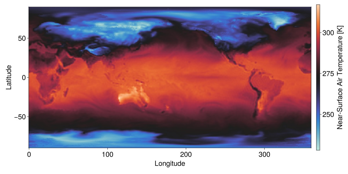
Wintri Projection
Some transformations
δlon = (lon_d[2] - lon_d[1])/2
nlon = lon_d .- 180 .+ δlon
ndata = circshift(data_d, (192,1))
and add Coastlines with GeoMakie.coastlines(),
fig = Figure(;size=(1200,600))
ax = GeoAxis(fig[1,1])
surface!(ax, nlon, lat_d, ndata; colormap = :seaborn_icefire_gradient, shading=false)
cl=lines!(ax, GeoMakie.coastlines(), color = :white, linewidth=0.85)
translate!(cl, 0, 0, 1000)
fig
Moll projection
fig = Figure(; size=(1200,600))
ax = GeoAxis(fig[1,1]; dest = "+proj=moll")
surface!(ax, nlon, lat_d, ndata; colormap = :seaborn_icefire_gradient, shading=false)
cl=lines!(ax, GeoMakie.coastlines(), color = :white, linewidth=0.85)
translate!(cl, 0, 0, 1000)
fig
3D sphere plot
using GLMakie
using GLMakie.GeometryBasics
GLMakie.activate!()

ds = replace(ndata, missing =>NaN)
sphere = uv_normal_mesh(Tesselation(Sphere(Point3f(0), 1), 128))

fig = Figure(backgroundcolor=:grey25, size=(500,500))
ax = LScene(fig[1,1], show_axis=false)
mesh!(ax, sphere; color = ds'[end:-1:1,:], shading=false,
    colormap = :seaborn_icefire_gradient)
zoom!(ax.scene, cameracontrols(ax.scene), 0.5)
rotate!(ax.scene, 2.5)
fig
AlgebraOfGraphics.jl
INFO
From DimensionalData docs :
AlgebraOfGraphics.jl is a high-level plotting library built on top of Makie.jl that provides a declarative algebra for creating complex visualizations, similar to ggplot2's "grammar of graphics" in R. It allows you to construct plots using algebraic operations like * and +, making it easy to create sophisticated graphics with minimal code.
using YAXArrays, Zarr, Dates
using GLMakie
using AlgebraOfGraphics
using GLMakie.GeometryBasics
GLMakie.activate!()
let's continue using the cmip6 dataset
store ="gs://cmip6/CMIP6/ScenarioMIP/DKRZ/MPI-ESM1-2-HR/ssp585/r1i1p1f1/3hr/tas/gn/v20190710/"
g = open_dataset(zopen(store, consolidated=true))
c = g["tas"];
and let's focus on the first time step:
dim_data = readcubedata(c[time=1]); # read into memory first!and now plot
data(dim_data) * mapping(:lon, :lat; color=Symbol("Near-Surface Air Temperature")) * visual(Scatter) |> draw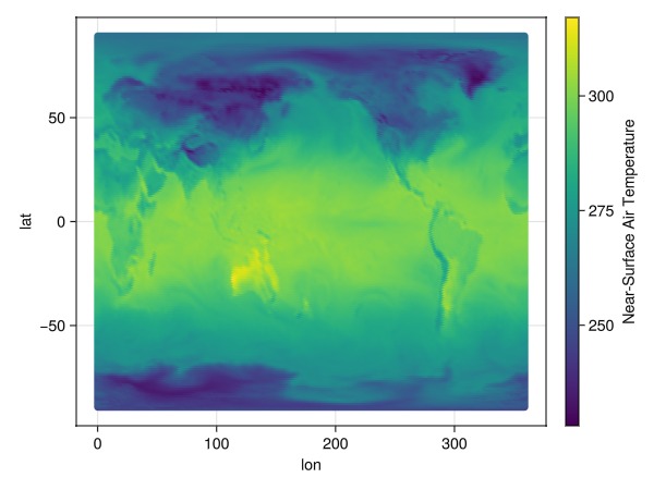
WARNING
Note that we are using a Scatter type per point and not the Heatmap one. There are workarounds for this, albeit cumbersome, so for now, let's keep this simpler syntax in mind along with the current approach being used.
set other attributes
plt = data(dim_data) * mapping(:lon, :lat; color=Symbol("Near-Surface Air Temperature"))
draw(plt * visual(Scatter, marker=:rect), scales(Color = (; colormap = :plasma));
    axis = (width = 600, height = 400, limits=(0, 360, -90, 90)))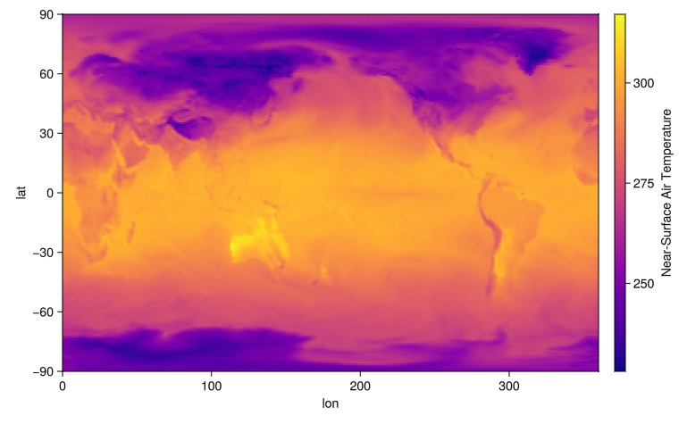
Faceting
For this let's consider more time steps from our dataset:
using Dates
dim_time = c[time=DateTime("2015-01-01") .. DateTime("2015-01-01T21:00:00")] # subset 7 t steps
┌ 384×192×7 YAXArray{Float32, 3} Near-Surface Air Temperature ┐
├─────────────────────────────────────────────────────────────┴────────── dims ┐
↓ lon Sampled{Float64} 0.0:0.9375:359.0625 ForwardOrdered Regular Points,
→ lat Sampled{Float64} [-89.28422753251364, …, 89.28422753251364] ForwardOrdered Irregular Points,
↗ time Sampled{DateTime} [DateTime("2015-01-01T03:00:00"), …, DateTime("2015-01-01T21:00:00")] ForwardOrdered Irregular Points
├──────────────────────────────────────────────────────────────────── metadata ┤
Dict{String, Any} with 10 entries:
"units" => "K"
"history" => "2019-07-21T06:26:13Z altered by CMOR: Treated scalar dime…
"name" => "tas"
"cell_methods" => "area: mean time: point"
"cell_measures" => "area: areacella"
"long_name" => "Near-Surface Air Temperature"
"coordinates" => "height"
"standard_name" => "air_temperature"
"_FillValue" => 1.0f20
"comment" => "near-surface (usually, 2 meter) air temperature"
├─────────────────────────────────────────────────────────────── loaded lazily ┤
data size: 1.97 MB
└──────────────────────────────────────────────────────────────────────────────┘dim_time = readcubedata(dim_time); # read into memory first!plt = data(dim_time) * mapping(:lon, :lat; color=Symbol("Near-Surface Air Temperature"), layout = :time => nonnumeric)
draw(plt * visual(Scatter, marker=:rect))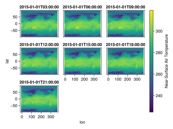
again, let's add some additional attributes
plt = data(dim_time) * mapping(:lon, :lat; color=Symbol("Near-Surface Air Temperature"),
    layout = :time => nonnumeric)
draw(plt * visual(Scatter, marker=:rect), scales(Color = (; colormap = :magma));
    axis = (; limits=(0, 360, -90, 90)),
    figure=(; size=(900,600)))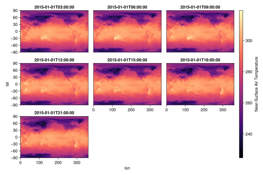
most Makie plot functions should work. See lines for example
plt = data(dim_data[lon=50..100]) * mapping(:lat, Symbol("Near-Surface Air Temperature") => "tas";
    color=Symbol("Near-Surface Air Temperature") => "tas")
draw(plt * visual(Lines); figure=(; size=(650,400)))
or faceting them
plt = data(dim_data[lon=50..59]) * mapping(:lat, Symbol("Near-Surface Air Temperature") => "tas";
    color=Symbol("Near-Surface Air Temperature") => "tas",
    layout = :lon => nonnumeric)
draw(plt * visual(Lines); figure=(; size=(650,400)))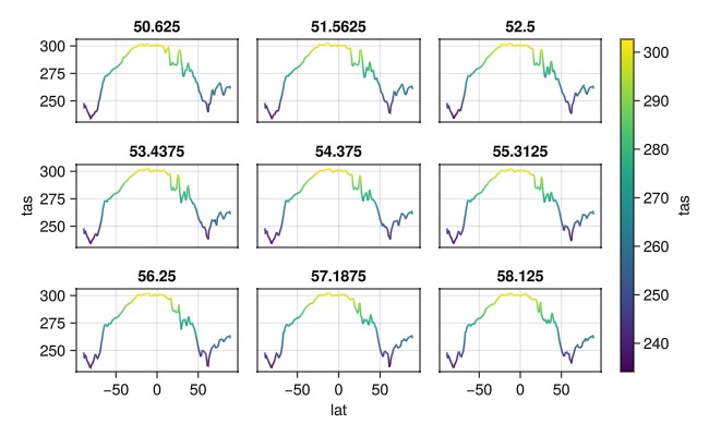
Time series
For this, let's load a little bit more of time steps
dim_series = c[time=DateTime("2015-01-01") .. DateTime("2015-01-04"), lon = 150 .. 157, lat = 0..1] |> readcubedata┌ 8×1×24 YAXArray{Float32, 3} Near-Surface Air Temperature ┐
├──────────────────────────────────────────────────────────┴───────────── dims ┐
↓ lon Sampled{Float64} 150.0:0.9375:156.5625 ForwardOrdered Regular Points,
→ lat Sampled{Float64} [0.4675308904227747] ForwardOrdered Irregular Points,
↗ time Sampled{DateTime} [DateTime("2015-01-01T03:00:00"), …, DateTime("2015-01-04T00:00:00")] ForwardOrdered Irregular Points
├──────────────────────────────────────────────────────────────────── metadata ┤
Dict{String, Any} with 10 entries:
"units" => "K"
"history" => "2019-07-21T06:26:13Z altered by CMOR: Treated scalar dime…
"name" => "tas"
"cell_methods" => "area: mean time: point"
"cell_measures" => "area: areacella"
"long_name" => "Near-Surface Air Temperature"
"coordinates" => "height"
"standard_name" => "air_temperature"
"_FillValue" => 1.0f20
"comment" => "near-surface (usually, 2 meter) air temperature"
├──────────────────────────────────────────────────────────── loaded in memory ┤
data size: 768.0 bytes
└──────────────────────────────────────────────────────────────────────────────┘and plot
plt = data(dim_series) * mapping(:time, Symbol("Near-Surface Air Temperature") => "tas"; color=:lon => nonnumeric)
draw(plt * visual(ScatterLines), scales(Color = (; palette = :tableau_colorblind));
    figure=(; size=(800,400)))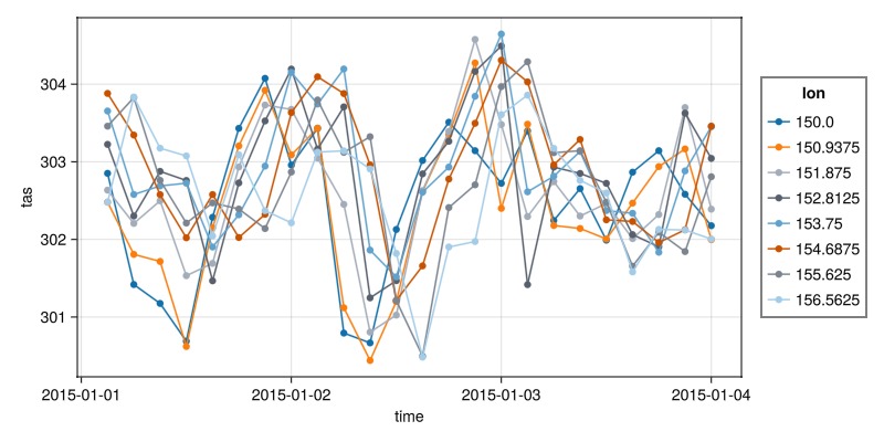
Analysis
Basic statistical analysis can also be done, for example:
specs = data(dim_data[lat=50..55]) * mapping(:lon, Symbol("Near-Surface Air Temperature") => "tas"; color=:lat => nonnumeric)
specs *= (smooth() + visual(Scatter))
draw(specs;  figure=(; size=(700,400)))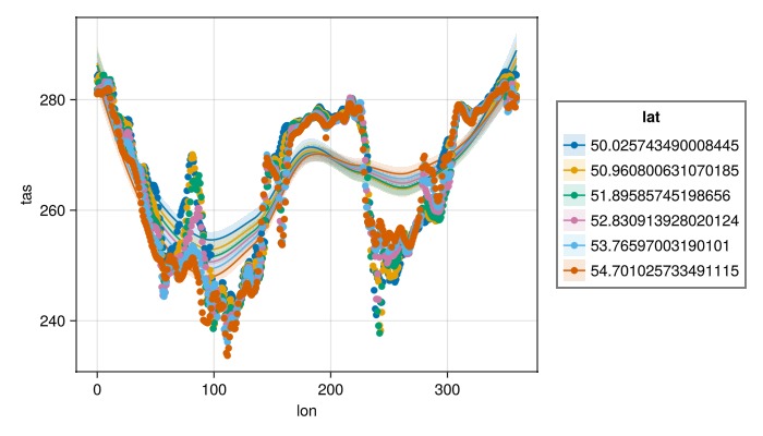
For more, visit AlgebraOfGraphics.jl.