Mean Seasonal Cycle for a sigle pixel
julia
using CairoMakie
CairoMakie.activate!()
using Dates
using Statistics
We define the data span. For simplicity, three non-leap years were selected.
julia
t =  Date("2021-01-01"):Day(1):Date("2023-12-31")
NpY = 33and create some seasonal dummy data
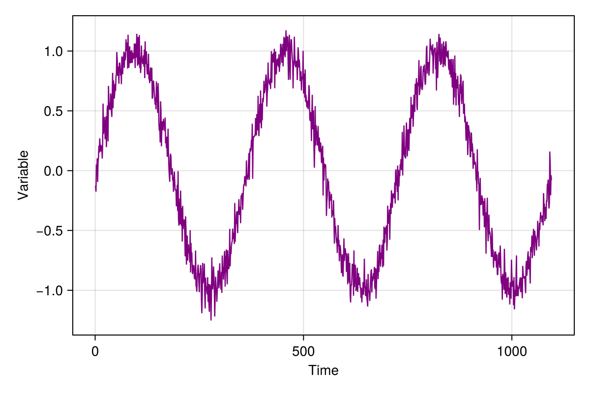
julia
x = repeat(range(0, 2π, length=365), NpY)
var = @. sin(x) + 0.1 * randn()
julia
lines(1:length(t), var; color = :purple, linewidth=1.25,
    axis=(; xlabel="Time", ylabel="Variable"),
    figure = (; resolution = (600,400))
    )
Currently makie doesn't support time axis natively, but the following function can do the work for now.
julia
function time_ticks(dates; frac=8)
    tempo = string.(dates)
    lentime = length(tempo)
    slice_dates = range(1, lentime, step=lentime ÷ frac)
    return slice_dates, tempo[slice_dates]
end
xpos, ticks = time_ticks(t; frac=8)
In order to apply the previous output, we split the plotting function into his 3 components, figure, axis and plotted object, namely
julia
fig, ax, obj = lines(1:length(t), var; color = :purple, linewidth=1.25,
    axis=(; xlabel="Time", ylabel="Variable"),
    figure = (; resolution = (600,400))
    )
ax.xticks = (xpos, ticks)
ax.xticklabelrotation = π / 4
ax.xticklabelalign = (:right, :center)
fig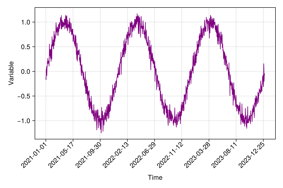
Define the cube
julia
julia> using YAXArrays, DimensionalData

julia> axes = (Dim{:Time}(t),)
↓ Time Date("2021-01-01"):Dates.Day(1):Date("2023-12-31")julia
julia> c = YAXArray(axes, var)╭──────────────────────────────────╮
│ 1095-element YAXArray{Float64,1} │
├──────────────────────────────────┴───────────────────────────────────── dims ┐
↓ Time Sampled{Date} Date("2021-01-01"):Dates.Day(1):Date("2023-12-31") ForwardOrdered Regular Points
├──────────────────────────────────────────────────────────────────── metadata ┤
Dict{String, Any}()
├─────────────────────────────────────────────────────────────────── file size ┤
file size: 8.55 KB
└──────────────────────────────────────────────────────────────────────────────┘Let's calculate the mean seasonal cycle of our dummy variable 'var'
julia
function mean_seasonal_cycle(c; ndays = 365)
    ## filterig by month-day
    monthday = map(x->Dates.format(x, "u-d"), collect(c.Time))
    datesid = unique(monthday)
    ## number of years
    NpY = Int(size(monthday,1)/ndays)
    idx = Int.(zeros(ndays, NpY))
    ## get the day-month indices for data subsetting
    for i in 1:ndays
        idx[i,:] = Int.(findall(x-> x == datesid[i], monthday))
    end
    ## compute the mean seasonal cycle
    mscarray = map(x->var[x], idx)
    msc = mapslices(mean, mscarray, dims=2)
    return msc
end

msc = mean_seasonal_cycle(c);
365×1 Matrix{Float64}:
-0.0826869939842561
-0.055917525181167715
0.05052340559150543
0.08451614708601285
0.010386935648898343
0.03711777134472371
0.19462641156452606
0.07781860783033945
0.19742778432205824
0.18004518550743445
⋮
-0.059007514969215934
-0.1596971775489893
-0.13864020025665416
-0.1676346860512412
0.03895957649357166
-0.10988958616474735
-0.037611457001786114
-0.07799964128473318
-0.04724062714352991TODO: Apply the new groupby funtion from DD
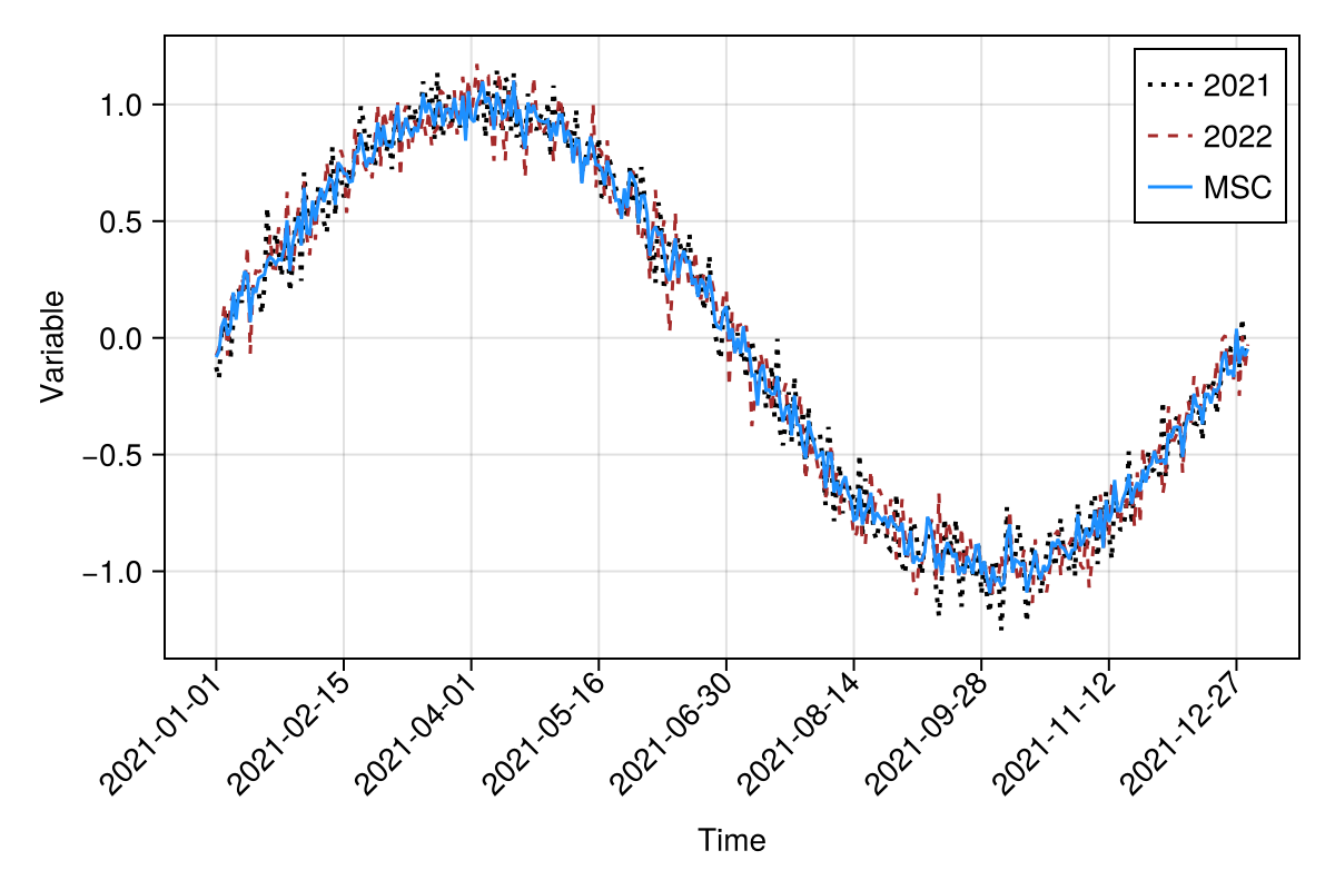
Plot results: mean seasonal cycle
julia
xpos, ticks = time_ticks(t[1:365]; frac=8)

fig, ax, obj = lines(1:365, var[1:365]; label="2021", color=:black,
    linewidth=2.0, linestyle=:dot,
    axis = (;  xlabel="Time", ylabel="Variable"),
    figure=(; size = (600,400))
    )
lines!(1:365, var[366:730], label="2022", color=:brown,
    linewidth=1.5, linestyle=:dash
    )
lines!(1:365, msc[:,1]; label="MSC", color=:dodgerblue, lw=2.5)
axislegend()
ax.xticks = (xpos, ticks)
ax.xticklabelrotation = π / 4
ax.xticklabelalign = (:right, :center)
fig
current_figure()