Plot YAXArrays

This section describes how to visualize YAXArrays. See also the Plotting maps tutorial to plot geospatial data. All plotting capabilities of AbstractDimArray apply to a YAXArrays as well, because every YAXArray is also an AbstractDimArray.

Plot a YAXArrray

Create a simple YAXArray:

using CairoMakie
using YAXArrays
using DimensionalData

data = collect(reshape(1:20, 4, 5))
axlist = (X(1:4), Y(1:5))
a = YAXArray(axlist, data)

┌ 4×5 YAXArray{Int64, 2} ┐
├────────────────────────┴───────────────────────── dims ┐
  ↓ X Sampled{Int64} 1:4 ForwardOrdered Regular Points,
  → Y Sampled{Int64} 1:5 ForwardOrdered Regular Points
├────────────────────────────────────── loaded in memory ┤
  data size: 160.0 bytes
└────────────────────────────────────────────────────────┘

Plot the entire array:

plot(a)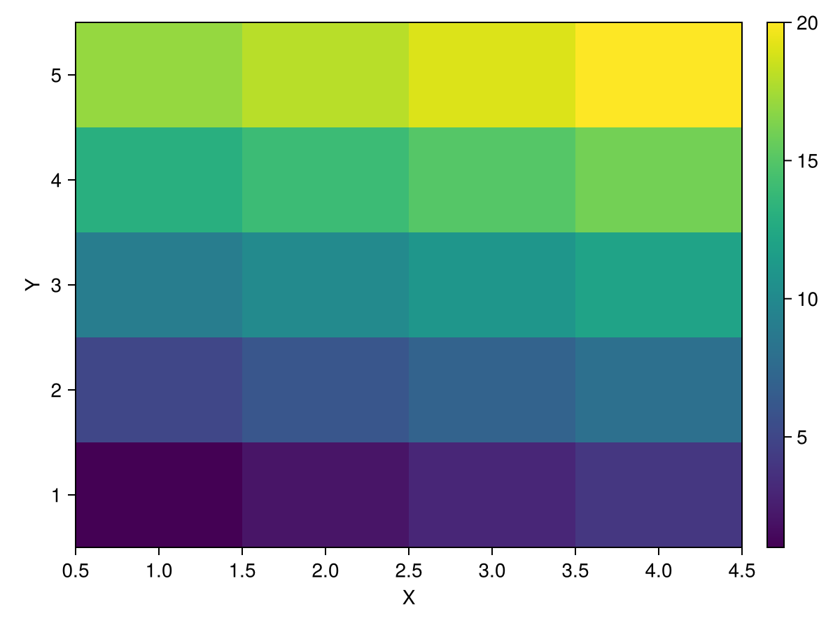

This will plot a heatmap, because the array is a matrix.

Plot the first column:

plot(a[Y=1])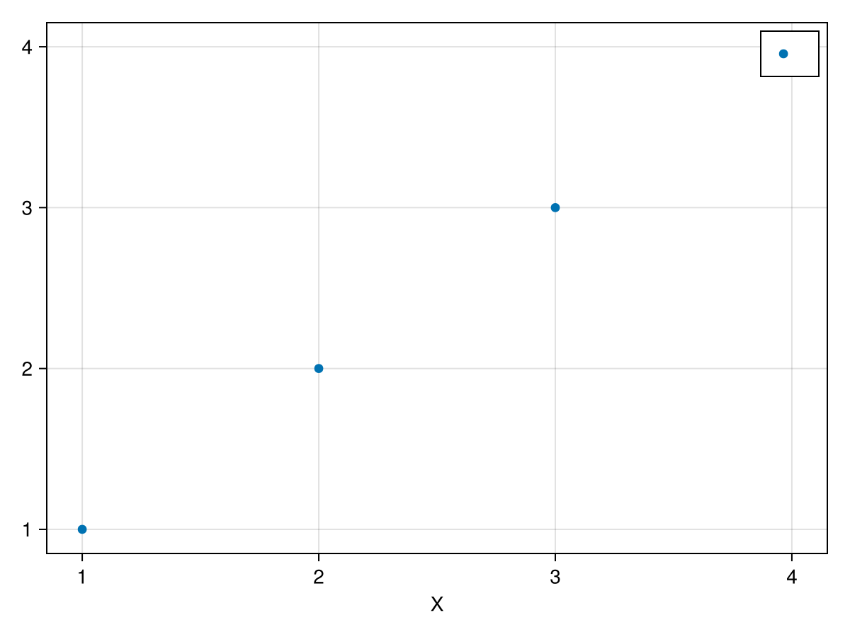

This results in a scatter plot, because the subarray is a vector.

Plot a YAXArrray with CF conventions

Climate and Forecast Metadata Conventions are used to generate appropriate labels for the plot whenever possible. This requires the YAXArray to have metadata properties like standard_name and units.

Get a Dataset with CF meta data:

using NetCDF
using Downloads: download

path = download("https://archive.unidata.ucar.edu/software/netcdf/examples/tos_O1_2001-2002.nc", "example.nc")
ds = open_dataset(path)

YAXArray Dataset
Shared Axes: 
  (↓ lon Sampled{Float64} 1.0:2.0:359.0 ForwardOrdered Regular Points,
  → lat Sampled{Float64} -79.5:1.0:89.5 ForwardOrdered Regular Points,
  ↗ time Sampled{CFTime.DateTime360Day{CFTime.Period{Float64, Val{86400}(), Val{0}()}, Val{(2001, 1, 1)}()}} [DateTime360Day(2001-01-16T00:00:00), …, DateTime360Day(2002-12-16T00:00:00)] ForwardOrdered Irregular Points)

Variables: 
tos

Properties: Dict{String, Any}("cmor_version" => 0.96f0, "references" => "Dufresne et al, Journal of Climate, 2015, vol XX, p 136", "realization" => 1, "Conventions" => "CF-1.0", "contact" => "Sebastien Denvil, sebastien.denvil@ipsl.jussieu.fr", "history" => "YYYY/MM/JJ: data generated; YYYY/MM/JJ+1 data transformed  At 16:37:23 on 01/11/2005, CMOR rewrote data to comply with CF standards and IPCC Fourth Assessment requirements", "table_id" => "Table O1 (13 November 2004)", "source" => "IPSL-CM4_v1 (2003) : atmosphere : LMDZ (IPSL-CM4_IPCC, 96x71x19) ; ocean ORCA2 (ipsl_cm4_v1_8, 2x2L31); sea ice LIM (ipsl_cm4_v", "title" => "IPSL  model output prepared for IPCC Fourth Assessment SRES A2 experiment", "experiment_id" => "SRES A2 experiment"…)

Plot the first time step of the sea surface temperature with CF metadata:

plot(ds.tos[time=1])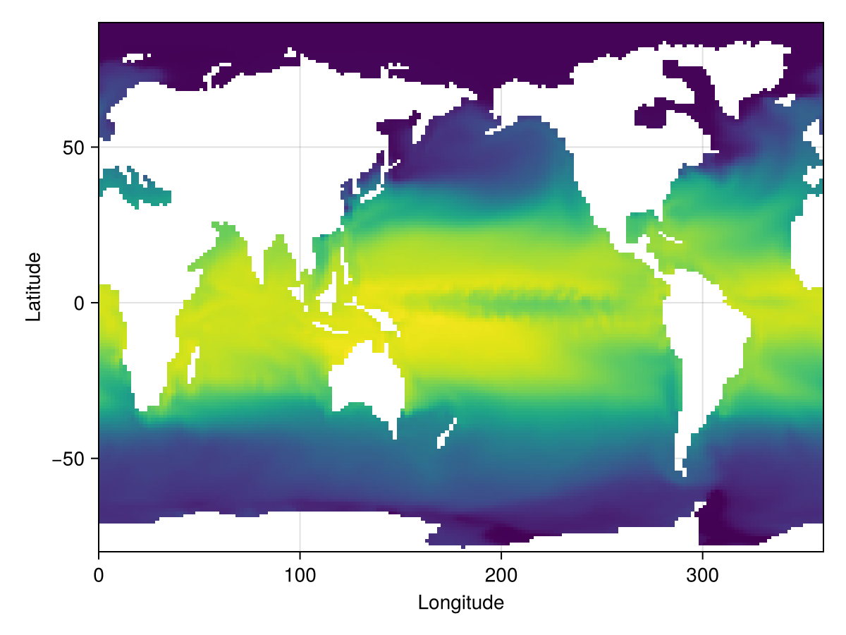

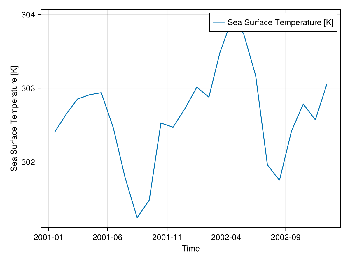
Time in Climate and Forecasting (CF) conventions requires conversion before plotting, e.g., to plot the sea surface temperature over time at a given location (e.g. the null island):

a = ds.tos[lon = Near(0), lat = Near(0)]
times = Ti(map(x -> DateTime(string(x)), a.time.val))
a = YAXArray((times,), collect(a.data), a.properties)

┌ 24-element YAXArray{Union{Missing, Float32}, 1} Sea Surface Temperature ┐
├─────────────────────────────────────────────────────────────────────────┴ dims ┐
  ↓ Ti Sampled{DateTime} [DateTime("2001-01-16T00:00:00"), …, DateTime("2002-12-16T00:00:00")] ForwardOrdered Irregular Points
├──────────────────────────────────────────────────────────────────── metadata ┤
  Dict{String, Any} with 10 entries:
  "units"          => "K"
  "missing_value"  => 1.0f20
  "history"        => " At   16:37:23 on 01/11/2005: CMOR altered the data in t…
  "cell_methods"   => "time: mean (interval: 30 minutes)"
  "name"           => "tos"
  "long_name"      => "Sea Surface Temperature"
  "original_units" => "degC"
  "standard_name"  => "sea_surface_temperature"
  "_FillValue"     => 1.0f20
  "original_name"  => "sosstsst"
├──────────────────────────────────────────────────────────── loaded in memory ┤
  data size: 96.0 bytes
└──────────────────────────────────────────────────────────────────────────────┘

plot(a)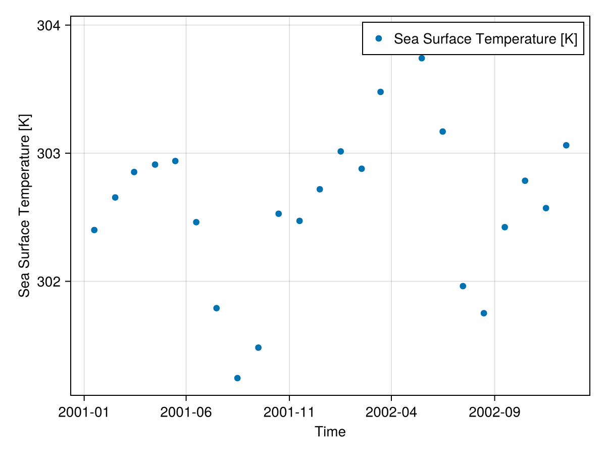

Or as as an explicit line plot:

lines(a)