Mean Seasonal Cycle for a sigle pixel
julia
using CairoMakie
CairoMakie.activate!()
using Dates
using Statistics
We define the data span. For simplicity, three non-leap years were selected.
julia
t =  Date("2021-01-01"):Day(1):Date("2023-12-31")
NpY = 33and create some seasonal dummy data
julia
x = repeat(range(0, 2π, length=365), NpY)
var = @. sin(x) + 0.1 * randn()
julia
lines(1:length(t), var; color = :purple, linewidth=1.25,
    axis=(; xlabel="Time", ylabel="Variable"),
    figure = (; resolution = (600,400))
    )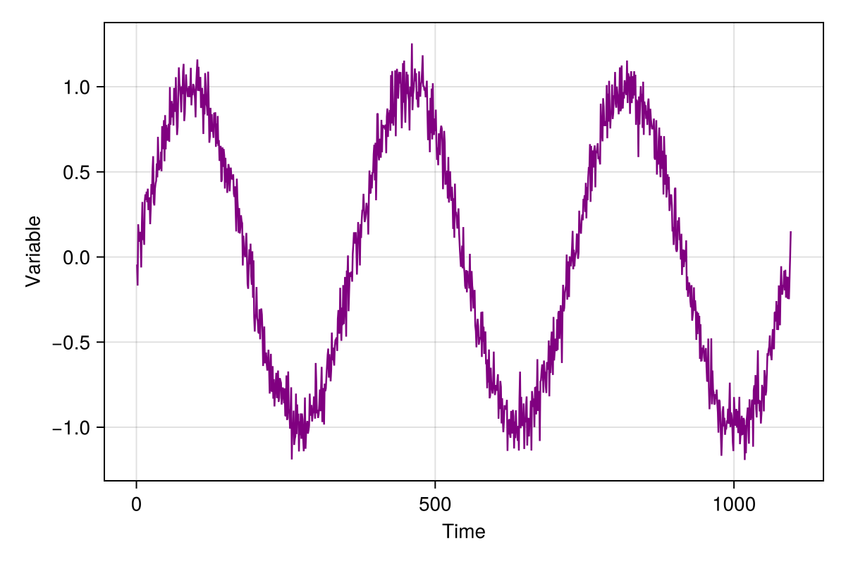
Currently makie doesn't support time axis natively, but the following function can do the work for now.
julia
function time_ticks(dates; frac=8)
    tempo = string.(dates)
    lentime = length(tempo)
    slice_dates = range(1, lentime, step=lentime ÷ frac)
    return slice_dates, tempo[slice_dates]
end
xpos, ticks = time_ticks(t; frac=8)
In order to apply the previous output, we split the plotting function into his 3 components, figure, axis and plotted object, namely
julia
fig, ax, obj = lines(1:length(t), var; color = :purple, linewidth=1.25,
    axis=(; xlabel="Time", ylabel="Variable"),
    figure = (; resolution = (600,400))
    )
ax.xticks = (xpos, ticks)
ax.xticklabelrotation = π / 4
ax.xticklabelalign = (:right, :center)
fig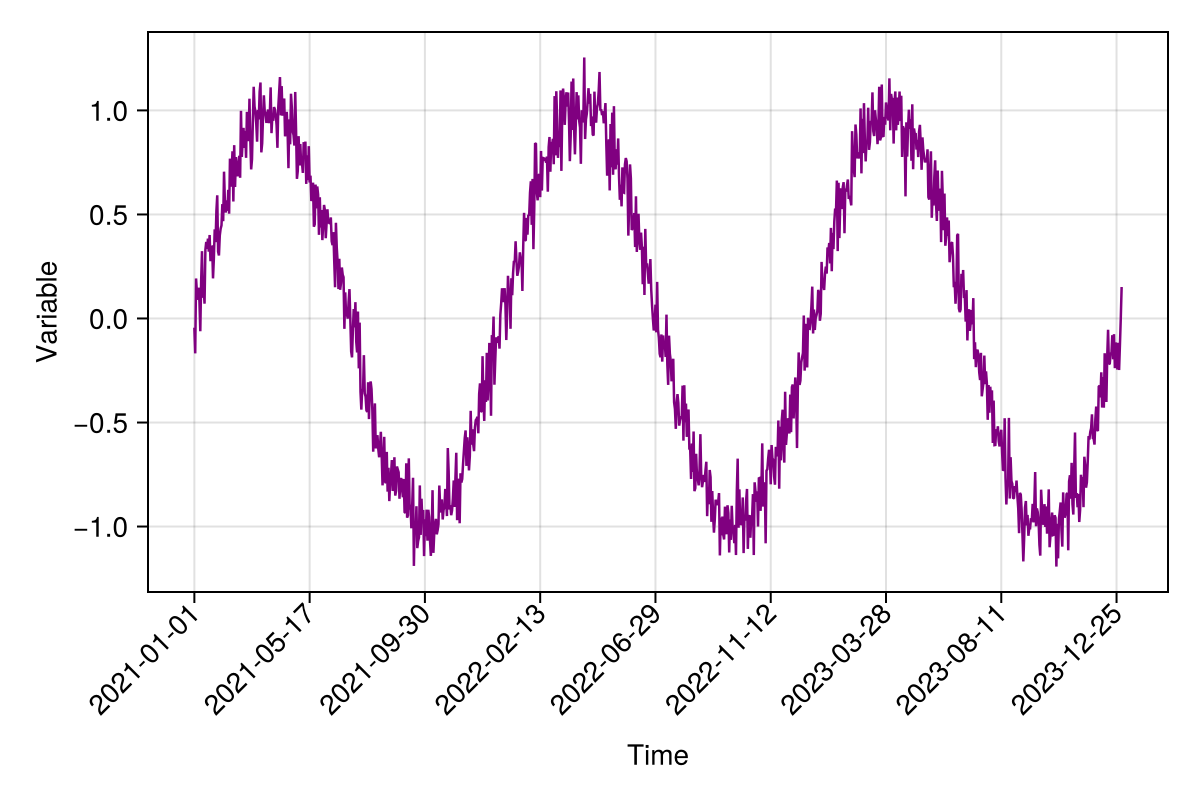
Define the cube
julia
julia> using YAXArrays, DimensionalData

julia> axes = (Dim{:Time}(t),)
↓ Time Date("2021-01-01"):Dates.Day(1):Date("2023-12-31")julia
julia> c = YAXArray(axes, var)╭──────────────────────────────────╮
│ 1095-element YAXArray{Float64,1} │
├──────────────────────────────────┴───────────────────────────────────── dims ┐
↓ Time Sampled{Date} Date("2021-01-01"):Dates.Day(1):Date("2023-12-31") ForwardOrdered Regular Points
├──────────────────────────────────────────────────────────────────── metadata ┤
Dict{String, Any}()
├─────────────────────────────────────────────────────────────────── file size ┤
file size: 8.55 KB
└──────────────────────────────────────────────────────────────────────────────┘Let's calculate the mean seasonal cycle of our dummy variable 'var'
julia
function mean_seasonal_cycle(c; ndays = 365)
    ## filterig by month-day
    monthday = map(x->Dates.format(x, "u-d"), collect(c.Time))
    datesid = unique(monthday)
    ## number of years
    NpY = Int(size(monthday,1)/ndays)
    idx = Int.(zeros(ndays, NpY))
    ## get the day-month indices for data subsetting
    for i in 1:ndays
        idx[i,:] = Int.(findall(x-> x == datesid[i], monthday))
    end
    ## compute the mean seasonal cycle
    mscarray = map(x->var[x], idx)
    msc = mapslices(mean, mscarray, dims=2)
    return msc
end

msc = mean_seasonal_cycle(c);
365×1 Matrix{Float64}:
-0.012689535514817496
0.007041149973688964
0.06731613697152088
0.008335004690090998
0.04299132526046814
0.12976794498840505
0.11682308096665517
0.06361687996374876
0.03996574028209171
0.17984271284557043
⋮
-0.15003310752070087
-0.08588085097677194
-0.1739275520791823
-0.1091596541503607
-0.10334128771843076
-0.09309797098972894
-0.02233588722394066
0.06964162211106674
0.14163601260787345TODO: Apply the new groupby funtion from DD
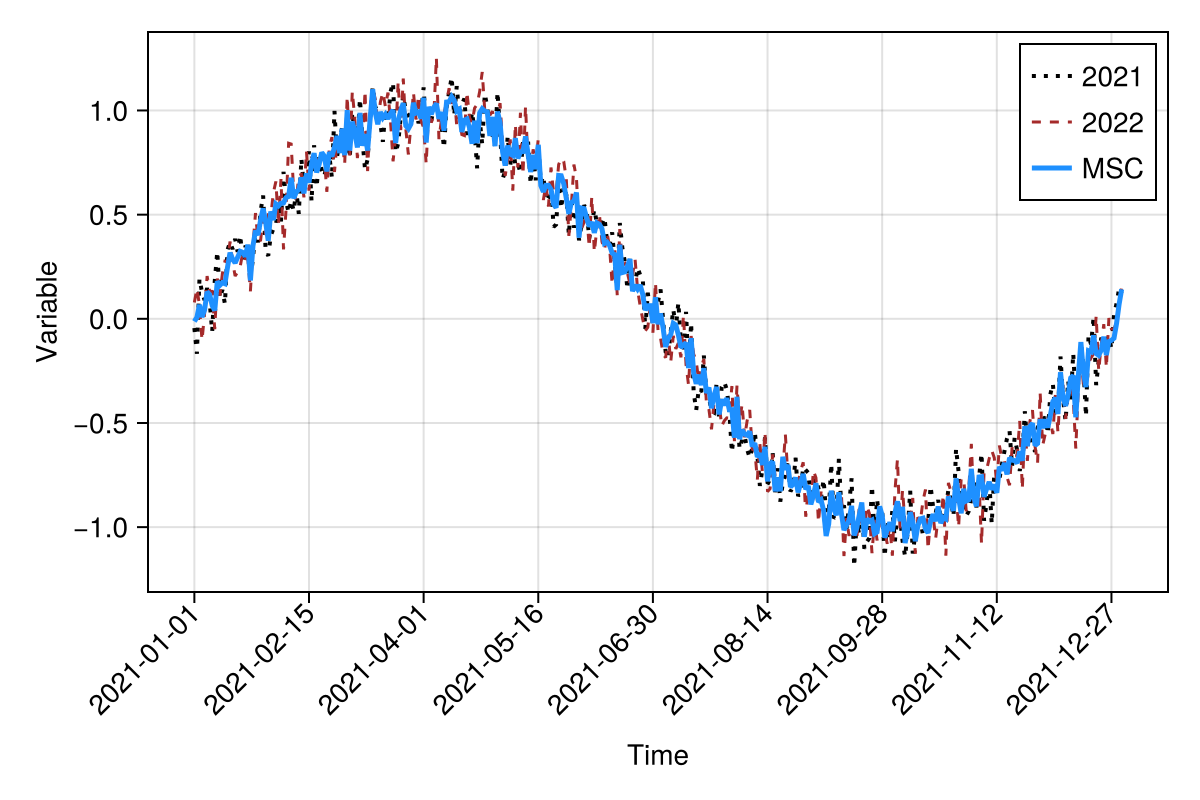
Plot results: mean seasonal cycle
julia
xpos, ticks = time_ticks(t[1:365]; frac=8)

fig, ax, obj = lines(1:365, var[1:365]; label="2021", color=:black,
    linewidth=2.0, linestyle=:dot,
    axis = (;  xlabel="Time", ylabel="Variable"),
    figure=(; size = (600,400))
    )
lines!(1:365, var[366:730], label="2022", color=:brown,
    linewidth=1.5, linestyle=:dash
    )
lines!(1:365, msc[:,1]; label="MSC", color=:dodgerblue, linewidth=2.5)
axislegend()
ax.xticks = (xpos, ticks)
ax.xticklabelrotation = π / 4
ax.xticklabelalign = (:right, :center)
fig
current_figure()