Frequently Asked Questions (FAQ)
The purpose of this section is to do a collection of small convinient pieces of code on how to do simple things.
Extract the axes names from a Cube
using YAXArrays
using DimensionalDatajulia> c = YAXArray(rand(10, 10, 5))╭─────────────────────────────╮
│ 10×10×5 YAXArray{Float64,3} │
├─────────────────────────────┴────────────────────────────────── dims ┐
↓ Dim_1 Sampled{Int64} Base.OneTo(10) ForwardOrdered Regular Points,
→ Dim_2 Sampled{Int64} Base.OneTo(10) ForwardOrdered Regular Points,
↗ Dim_3 Sampled{Int64} Base.OneTo(5) ForwardOrdered Regular Points
├──────────────────────────────────────────────────────────── metadata ┤
Dict{String, Any}()
├─────────────────────────────────────────────────────────── file size ┤
file size: 3.91 KB
└──────────────────────────────────────────────────────────────────────┘julia> caxes(c) # former way of doing it↓ Dim_1 Sampled{Int64} Base.OneTo(10) ForwardOrdered Regular Points,
→ Dim_2 Sampled{Int64} Base.OneTo(10) ForwardOrdered Regular Points,
↗ Dim_3 Sampled{Int64} Base.OneTo(5) ForwardOrdered Regular PointsWARNING
To get the axes of a YAXArray use the dims function instead of the caxes function
julia> dims(c)↓ Dim_1 Sampled{Int64} Base.OneTo(10) ForwardOrdered Regular Points,
→ Dim_2 Sampled{Int64} Base.OneTo(10) ForwardOrdered Regular Points,
↗ Dim_3 Sampled{Int64} Base.OneTo(5) ForwardOrdered Regular PointsINFO
Also, use DD.rebuild(ax, values) instead of axcopy(ax, values) to copy an axes with the same name but different values.
Obtain values from axes and data from the cube
There are two options to collect values from axes. In this examples the axis ranges from 1 to 10.
These two examples bring the same result
collect(getAxis("Dim_1", c).val)
collect(c.axes[1].val)
10-element Vector{Int64}:
1
2
3
4
5
6
7
8
9
10to collect data from a cube works exactly the same as doing it from an array
julia> c[:, :, 1]╭───────────────────────────╮
│ 10×10 YAXArray{Float64,2} │
├───────────────────────────┴────────────────────────── dims ┐
↓ Dim_1 Sampled{Int64} 1:10 ForwardOrdered Regular Points,
→ Dim_2 Sampled{Int64} 1:10 ForwardOrdered Regular Points
├────────────────────────────────────────────────── metadata ┤
Dict{String, Any}()
├───────────────────────────────────────────────── file size ┤
file size: 800.0 bytes
└────────────────────────────────────────────────────────────┘How do I concatenate cubes
It is possible to concatenate several cubes that shared the same dimensions using the [concatenatecubes]@ref function.
Let's create two dummy cubes
using YAXArrays
axlist = (
    Dim{:time}(range(1, 20, length=20)),
    Dim{:lon}(range(1, 10, length=10)),
    Dim{:lat}(range(1, 5, length=15))
    )

data1 = rand(20, 10, 15)
ds1 = YAXArray(axlist, data1)

data2 = rand(20, 10, 15)
ds2 = YAXArray(axlist, data2)
Now we can concatenate ds1 and ds2:
julia> dsfinal = concatenatecubes([ds1, ds2], Dim{:Variables}(["var1", "var2"]))╭────────────────────────────────╮
│ 20×10×15×2 YAXArray{Float64,4} │
├────────────────────────────────┴─────────────────────────────────────── dims ┐
↓ time Sampled{Float64} 1.0:1.0:20.0 ForwardOrdered Regular Points,
→ lon Sampled{Float64} 1.0:1.0:10.0 ForwardOrdered Regular Points,
↗ lat Sampled{Float64} 1.0:0.2857142857142857:5.0 ForwardOrdered Regular Points,
⬔ Variables Categorical{String} ["var1", "var2"] ForwardOrdered
├──────────────────────────────────────────────────────────────────── metadata ┤
Dict{String, Any}()
├─────────────────────────────────────────────────────────────────── file size ┤
file size: 46.88 KB
└──────────────────────────────────────────────────────────────────────────────┘How do I subset a Cube?
Let's start by creating a dummy cube. Define the time span of the cube
using Dates
t = Date("2020-01-01"):Month(1):Date("2022-12-31")Date("2020-01-01"):Dates.Month(1):Date("2022-12-01")create cube axes
axes = (Dim{:Lon}(1:10), Dim{:Lat}(1:10), Dim{:Time}(t))↓ Lon 1:10,
→ Lat 1:10,
↗ Time Date("2020-01-01"):Dates.Month(1):Date("2022-12-01")assign values to a cube
julia> c = YAXArray(axes, reshape(1:3600, (10, 10, 36)))╭────────────────────────────╮
│ 10×10×36 YAXArray{Int64,3} │
├────────────────────────────┴─────────────────────────────────────────── dims ┐
↓ Lon Sampled{Int64} 1:10 ForwardOrdered Regular Points,
→ Lat Sampled{Int64} 1:10 ForwardOrdered Regular Points,
↗ Time Sampled{Date} Date("2020-01-01"):Dates.Month(1):Date("2022-12-01") ForwardOrdered Regular Points
├──────────────────────────────────────────────────────────────────── metadata ┤
Dict{String, Any}()
├─────────────────────────────────────────────────────────────────── file size ┤
file size: 28.12 KB
└──────────────────────────────────────────────────────────────────────────────┘Now we subset the cube by any dimension.
Subset cube by years
julia> ctime = c[Time=Between(Date(2021,1,1), Date(2021,12,31))]╭────────────────────────────╮
│ 10×10×12 YAXArray{Int64,3} │
├────────────────────────────┴─────────────────────────────────────────── dims ┐
↓ Lon Sampled{Int64} 1:10 ForwardOrdered Regular Points,
→ Lat Sampled{Int64} 1:10 ForwardOrdered Regular Points,
↗ Time Sampled{Date} Date("2021-01-01"):Dates.Month(1):Date("2021-12-01") ForwardOrdered Regular Points
├──────────────────────────────────────────────────────────────────── metadata ┤
Dict{String, Any}()
├─────────────────────────────────────────────────────────────────── file size ┤
file size: 9.38 KB
└──────────────────────────────────────────────────────────────────────────────┘Subset cube by a specific date and date range
julia> ctime2 = c[Time=At(Date("2021-05-01"))]╭─────────────────────────╮
│ 10×10 YAXArray{Int64,2} │
├─────────────────────────┴────────────────────────── dims ┐
↓ Lon Sampled{Int64} 1:10 ForwardOrdered Regular Points,
→ Lat Sampled{Int64} 1:10 ForwardOrdered Regular Points
├──────────────────────────────────────────────── metadata ┤
Dict{String, Any}()
├─────────────────────────────────────────────── file size ┤
file size: 800.0 bytes
└──────────────────────────────────────────────────────────┘julia> ctime3 = c[Time=Date("2021-05-01") .. Date("2021-12-01")]╭───────────────────────────╮
│ 10×10×8 YAXArray{Int64,3} │
├───────────────────────────┴──────────────────────────────────────────── dims ┐
↓ Lon Sampled{Int64} 1:10 ForwardOrdered Regular Points,
→ Lat Sampled{Int64} 1:10 ForwardOrdered Regular Points,
↗ Time Sampled{Date} Date("2021-05-01"):Dates.Month(1):Date("2021-12-01") ForwardOrdered Regular Points
├──────────────────────────────────────────────────────────────────── metadata ┤
Dict{String, Any}()
├─────────────────────────────────────────────────────────────────── file size ┤
file size: 6.25 KB
└──────────────────────────────────────────────────────────────────────────────┘Subset cube by longitude and latitude
julia> clonlat = c[Lon=1 .. 5, Lat=5 .. 10] # check even numbers range, it is ommiting them╭──────────────────────────╮
│ 5×6×36 YAXArray{Int64,3} │
├──────────────────────────┴───────────────────────────────────────────── dims ┐
↓ Lon Sampled{Int64} 1:5 ForwardOrdered Regular Points,
→ Lat Sampled{Int64} 5:10 ForwardOrdered Regular Points,
↗ Time Sampled{Date} Date("2020-01-01"):Dates.Month(1):Date("2022-12-01") ForwardOrdered Regular Points
├──────────────────────────────────────────────────────────────────── metadata ┤
Dict{String, Any}()
├─────────────────────────────────────────────────────────────────── file size ┤
file size: 8.44 KB
└──────────────────────────────────────────────────────────────────────────────┘How do I apply map algebra?
Our next step is map algebra computations. This can be done effectively using the 'map' function. For example:
Multiplying cubes with only spatio-temporal dimensions
julia> map((x, y) -> x * y, ds1, ds2)╭──────────────────────────────╮
│ 20×10×15 YAXArray{Float64,3} │
├──────────────────────────────┴───────────────────────────────────────── dims ┐
↓ time Sampled{Float64} 1.0:1.0:20.0 ForwardOrdered Regular Points,
→ lon Sampled{Float64} 1.0:1.0:10.0 ForwardOrdered Regular Points,
↗ lat Sampled{Float64} 1.0:0.2857142857142857:5.0 ForwardOrdered Regular Points
├──────────────────────────────────────────────────────────────────── metadata ┤
Dict{String, Any}()
├─────────────────────────────────────────────────────────────────── file size ┤
file size: 23.44 KB
└──────────────────────────────────────────────────────────────────────────────┘Cubes with more than 3 dimensions
julia> map((x, y) -> x * y, dsfinal[Variables=At("var1")], dsfinal[Variables=At("var2")])╭──────────────────────────────╮
│ 20×10×15 YAXArray{Float64,3} │
├──────────────────────────────┴───────────────────────────────────────── dims ┐
↓ time Sampled{Float64} 1.0:1.0:20.0 ForwardOrdered Regular Points,
→ lon Sampled{Float64} 1.0:1.0:10.0 ForwardOrdered Regular Points,
↗ lat Sampled{Float64} 1.0:0.2857142857142857:5.0 ForwardOrdered Regular Points
├──────────────────────────────────────────────────────────────────── metadata ┤
Dict{String, Any}()
├─────────────────────────────────────────────────────────────────── file size ┤
file size: 23.44 KB
└──────────────────────────────────────────────────────────────────────────────┘To add some complexity, we will multiply each value for π and then divided for the sum of each time step. We will use the ds1 cube for this purpose.
julia> mapslices(ds1, dims=("Lon", "Lat")) do xin
           (xin * π) ./ maximum(skipmissing(xin))
       end
╭──────────────────────────────────────────────╮
│ 10×15×20 YAXArray{Union{Missing, Float64},3} │
├──────────────────────────────────────────────┴───────────────────────── dims ┐
↓ lon Sampled{Float64} 1.0:1.0:10.0 ForwardOrdered Regular Points,
→ lat Sampled{Float64} 1.0:0.2857142857142857:5.0 ForwardOrdered Regular Points,
↗ time Sampled{Float64} 1.0:1.0:20.0 ForwardOrdered Regular Points
├──────────────────────────────────────────────────────────────────── metadata ┤
Dict{String, Any}()
├─────────────────────────────────────────────────────────────────── file size ┤
file size: 23.44 KB
└──────────────────────────────────────────────────────────────────────────────┘How do I use the CubeTable function?
The function "CubeTable" creates an iterable table and the result is a DataCube. It is therefore very handy for grouping data and computing statistics by class. It uses OnlineStats.jl to calculate statistics, and weighted statistics can be calculated as well.
Here we will use the ds1 Cube defined previously and we create a mask for data classification.
Cube containing a mask with classes 1, 2 and 3.
julia> classes = YAXArray((getAxis("lon", dsfinal), getAxis("lat", dsfinal)), rand(1:3, 10, 15))╭─────────────────────────╮
│ 10×15 YAXArray{Int64,2} │
├─────────────────────────┴────────────────────────────────────────────── dims ┐
↓ lon Sampled{Float64} 1.0:1.0:10.0 ForwardOrdered Regular Points,
→ lat Sampled{Float64} 1.0:0.2857142857142857:5.0 ForwardOrdered Regular Points
├──────────────────────────────────────────────────────────────────── metadata ┤
Dict{String, Any}()
├─────────────────────────────────────────────────────────────────── file size ┤
file size: 1.17 KB
└──────────────────────────────────────────────────────────────────────────────┘using GLMakie
GLMakie.activate!()
# This is how our classification map looks like
fig, ax, obj = heatmap(classes;
colormap=Makie.Categorical(cgrad([:grey15, :orangered, :snow3])))
cbar = Colorbar(fig[1,2], obj)
fig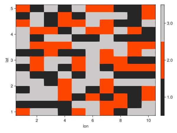
Now we define the input cubes that will be considered for the iterable table
t = CubeTable(values=ds1, classes=classes)Datacube iterator with 1 subtables with fields: (:values, :classes, :time, :lon, :lat)using DataFrames
using OnlineStats
## visualization of the CubeTable
c_tbl = DataFrame(t[1])
first(c_tbl, 5)In this line we calculate the Mean for each class
julia> fitcube = cubefittable(t, Mean, :values, by=(:classes))╭───────────────────────────────────────────────╮
│ 3-element YAXArray{Union{Missing, Float64},1} │
├───────────────────────────────────────────────┴────────────── dims ┐
↓ classes Sampled{Int64} [1, 2, 3] ForwardOrdered Irregular Points
├────────────────────────────────────────────────────────── metadata ┤
Dict{String, Any}()
├───────────────────────────────────────────────────────── file size ┤
file size: 24.0 bytes
└────────────────────────────────────────────────────────────────────┘We can also use more than one criteria for grouping the values. In the next example, the mean is calculated for each class and timestep.
julia> fitcube = cubefittable(t, Mean, :values, by=(:classes, :time))╭──────────────────────────────────────────╮
│ 3×20 YAXArray{Union{Missing, Float64},2} │
├──────────────────────────────────────────┴────────────────────── dims ┐
↓ classes Sampled{Int64} [1, 2, 3] ForwardOrdered Irregular Points,
→ time Sampled{Float64} 1.0:1.0:20.0 ForwardOrdered Regular Points
├───────────────────────────────────────────────────────────── metadata ┤
Dict{String, Any}()
├──────────────────────────────────────────────────────────── file size ┤
file size: 480.0 bytes
└───────────────────────────────────────────────────────────────────────┘How do I assing variable names to YAXArrays in a Dataset
One variable name
julia> ds = YAXArrays.Dataset(; (:a => YAXArray(rand(10)),)...)YAXArray Dataset
Shared Axes:
↓ Dim_1 Sampled{Int64} Base.OneTo(10) ForwardOrdered Regular Points
Variables:
aMultiple variable names
keylist = (:a, :b, :c)
varlist = (YAXArray(rand(10)), YAXArray(rand(10,5)), YAXArray(rand(2,5)))julia> ds = YAXArrays.Dataset(; (keylist .=> varlist)...)YAXArray Dataset
Shared Axes:
()
Variables:
a
↓ Dim_1 Sampled{Int64} Base.OneTo(10) ForwardOrdered Regular Points
b
↓ Dim_1 Sampled{Int64} Base.OneTo(10) ForwardOrdered Regular Points,
→ Dim_2 Sampled{Int64} Base.OneTo(5) ForwardOrdered Regular Points
c
↓ Dim_1 Sampled{Int64} Base.OneTo(2) ForwardOrdered Regular Points,
→ Dim_2 Sampled{Int64} Base.OneTo(5) ForwardOrdered Regular Points